📋 Project Overview
Central Theme
To investigate how environmental and geomorphological variables influence the diversity and distribution of marine macrophytes across three coastal islands of Santa Catarina, focusing on spatial mapping and habitat suitability modeling.
Context and Relevance
- Marine macrophytes are ecosystem engineers that sustain high coastal biodiversity.
- These communities respond to changes in temperature, water transparency, and substrate structure.
- The climate crisis and anthropogenic pressure increase the vulnerability of island habitats.
- The project integrates biological inventory, geoprocessing, and SDMs (models that estimate where species are most likely to occur) to support applied conservation.
The Problem the Project Addresses
There is still a lack of detailed and comparable maps showing where marine macrophytes occur on the coastal islands of Santa Catarina and how they respond to environmental changes. Without this foundation, it becomes harder to prioritize monitoring and plan conservation actions.
What Will Be Done in Practice
1) Field Survey
The team records species, abundance, and environmental conditions on the three islands using a standardized methodology to enable fair comparison.
2) Mapping and Modeling
Field data are integrated into maps and models to indicate the most favorable areas for macrophytes and priority areas for monitoring.
3) Applicable Deliverables
The project generates scientific and technical products that can be used by research, environmental management, and coastal monitoring planning.
Why Does This Matter for Non-Specialists?
- Helps identify the most sensitive marine areas that need protection.
- Improves the technical basis for public decisions on coastal conservation.
- Creates a comparable record to track changes over the years.
- Translates complex data into maps and useful information for different audiences.
Questions the Project Answers
- Which macrophyte species dominate each island and how do they vary with depth?
- Which habitat conditions favor greater occurrence and relative abundance?
- How to spatially represent priority zones for monitoring and management?
- How might warming scenarios shift areas of greatest habitat suitability?
How to Read This Presentation
- Study Areas: shows where the project takes place and why these islands were chosen.
- Objectives: clearly explains what the project aims to deliver.
- Methodology: details how data will be collected, analyzed, and transformed into maps.
- Products: presents the expected results for science and environmental management.
- Glossary: defines technical terms in accessible language.
- Timeline: shows when each stage will be carried out.
🗺️ Study Areas
Geographic Scope
Three coastal islands of Santa Catarina with a gradient of size, isolation, and anthropogenic pressure.
🟠 REBIO Marinha do Arvoredo
Centroid: 27°13'33"S, 48°21'56"W
Area: 17,131.72 ha
Status: Federal Conservation Unit
Distance from shore: ~15 km
Study depth range: 0–15 m
- Largest study area
- Conservation reference site
- Regulated diving
- High microhabitat heterogeneity
- Rocky substrate with rocky shores and high-energy zones
- Greater potential for internal ecological gradients
🔵 Ilha do Campeche
Centroid: 27°41'48"S, 48°27'55"W
Area: 76.19 ha
Status: Archaeological/Scenic Heritage
Distance from shore: ~1.5 km
Study depth range: 0–15 m
- Close proximity to the mainland
- High tourist pressure
- Good fieldwork accessibility
- Ideal environment to assess anthropogenic influence
- Mixed substrate (rocky/sandy) in distinct sectors
- Greater exposure to recreational use and boat traffic
🟢 Ilha Xavier
Centroid: 27°36'36"S, 48°23'11"W
Area: 16.98 ha
Status: No specific protection
Distance from shore: ~8 km
Study depth range: 0–15 m
- Smallest study area
- Group of islets
- Intermediate pressure conditions
- Least studied area in local literature
- Good sensitivity for detecting rapid changes
- Intermediate connectivity between mainland and Arvoredo
Complete Comparison of Study Areas
| Criterion | Arvoredo | Campeche | Xavier |
|---|---|---|---|
| Area (ha) | 17,131.72 | 76.19 | 16.98 |
| Relative size | ~1,000x larger than Xavier | Intermediate | Smallest in the gradient |
| Distance from shore | ~15 km | ~1.5 km | ~8 km |
| Protection status | Federal Conservation Unit (REBIO) | Archaeological/Scenic Heritage | No specific protection |
| Anthropogenic pressure | Low (regulated) | High | Moderate |
| Tourist pressure | Controlled | Intense in summer | Lower than Campeche |
| Logistical accessibility | More complex (vessel and weather window) | Simpler and faster | Intermediate |
| Degree of isolation | High | Low | Intermediate |
| Habitat complexity | High (multiple microenvironments) | Medium (contrasting sectors) | Medium/high at small scale |
| Dominant substrate | Rocky shores with high-energy zones | Rocky and sandy mosaic | Rocky shores and islets |
| Relevance for modeling | Reference for more preserved conditions | Reference for high anthropogenic influence | Reference for a small, understudied area |
| Role in study gradient | Extreme of largest area/isolation | Extreme of greatest human use/proximity | Intermediate connectivity point |
🎯 Selection Rationale
The selection of Arvoredo, Campeche, and Xavier was made to represent a realistic and comparable ecological gradient at a regional scale, enabling robust tests on macrophyte distribution and habitat suitability.
- Area gradient: strong contrast between large, medium, and small islands.
- Isolation gradient: variation in connectivity with the coast and between islands.
- Anthropogenic pressure gradient: from regulated use to intense tourist use.
- Different protection regimes: comparison between a federal conservation unit and areas without equivalent protection.
- Operational feasibility: a set with feasible logistics for repeated surveys and spatial modeling.
🗺️ Maps of the Study Areas
The maps below show the spatial basis used to compare Arvoredo, Campeche, and Xavier. These are the cartographic products providing the territorial context of the study.
How to use the interactive map: click the button below to open a dynamic view of the three study areas. On the map, you can switch basemaps, check the legend and cartographic metadata, use both the graphic and numeric scales, and zoom in/out to explore spatial details of each island.
Open interactive map of study areas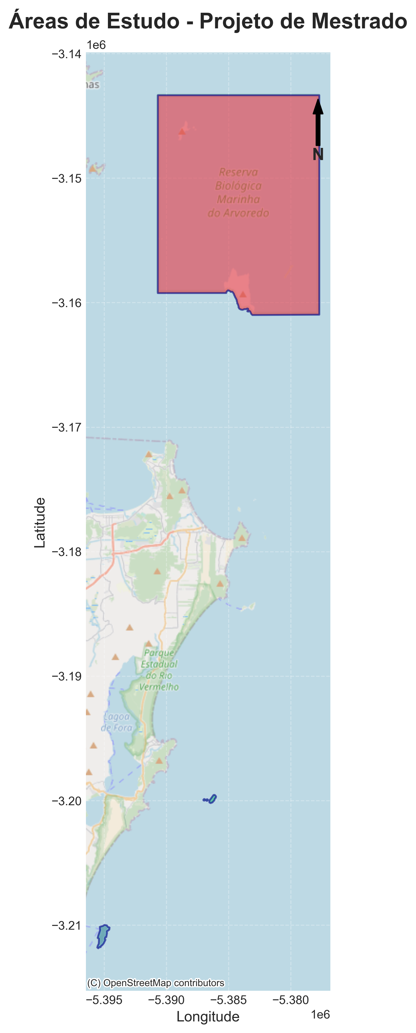
Reference map of the three island study areas.
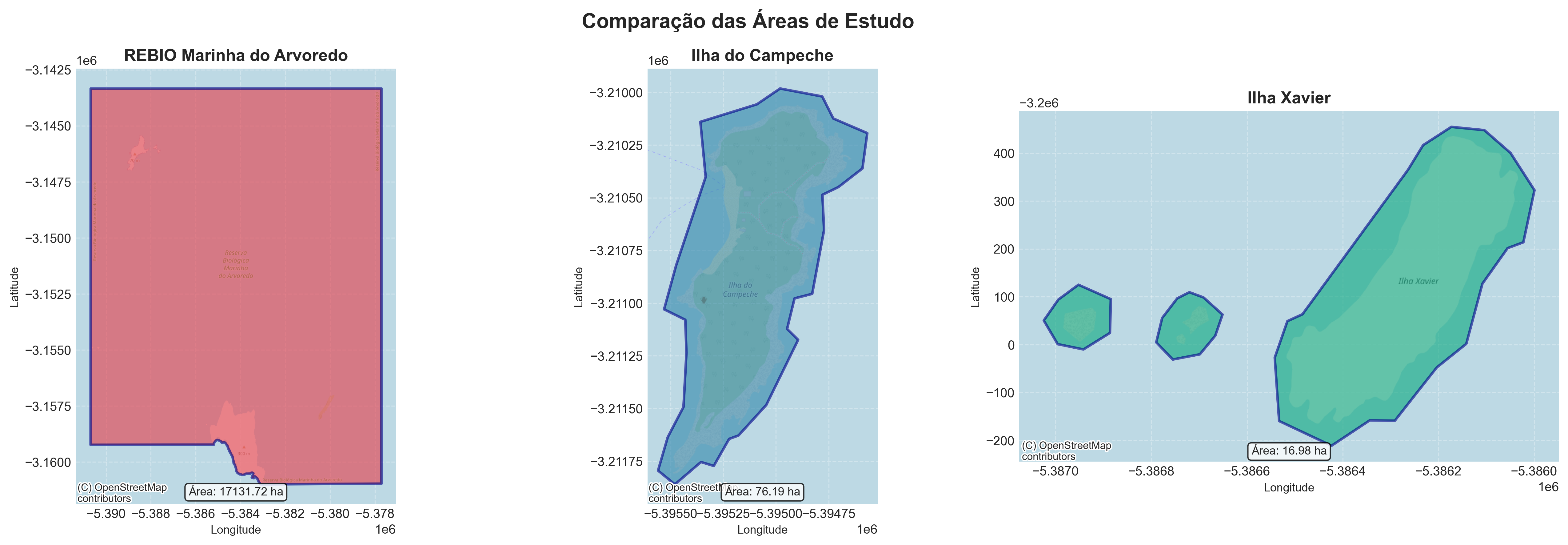
Spatial comparison of REBIO Arvoredo, Campeche, and Xavier.
🎯 Objectives
General Objective
To assess the diversity and spatial distribution of marine macrophyte communities in Ilha do Campeche, Ilha Xavier, and REBIO Marinha do Arvoredo, correlating biological patterns with environmental and geomorphological variables to generate habitat suitability models.
Specific Objectives
1 Floristic Inventory
Conduct an inventory of macrophytes in the 0–15 m depth range.
2 GIS Mapping
Map spatial distribution and relative abundance using geoprocessing.
3 Drone Photogrammetry
Generate orthophotos and surface models to refine habitat mapping.
4 Abiotic Variables
Characterize rocky substrate and local variables such as water transparency.
5 Habitat Modeling
Build a habitat suitability index (HSI) and SDMs to estimate occurrence patterns (i.e., where species tend to be found).
6 Reference Collection
Consolidate a reference collection (herbarium) for long-term monitoring.
🔬 Methodology
Methodology in Plain Language
The study logic is straightforward: measure macrophytes in the field, record environmental conditions, and then transform that into maps and models to understand where each species is most likely to occur.
Methodological Flow Infographic
Connected visual summary: from field collection through to final conservation products.
Planning
Points, transects, and logistics.
Biological Sampling
Freediving/SCUBA, presence, abundance (DAFOR), and rocky shore collection.
Environmental Sampling
Depth, transparency, and substrate.
Photogrammetry
Orthophoto and DSM with RGB/multispectral.
GIS
Spatial data integration.
HSI + SDMs
Suitability and distribution modeling.
Validation
Field checks and performance metrics.
Final Products
Maps and synthesis for monitoring.
1) How the Study Will Be Conducted
Study type: comparison between three islands (Arvoredo, Campeche, and Xavier).
Depth range: 0 to 15 m.
Strategy: apply the same method across all three areas to allow fair comparisons.
2) Practical Steps (Step by Step)
| Step | What Will Be Done | Expected Outcome |
|---|---|---|
| Step 1 | Define sampling points, transects, and operational windows (tide/weather) for each island | Standardized fieldwork plan |
| Step 2 | Conduct underwater sampling by freediving (shallow sectors) and SCUBA diving (deeper sectors), with safety protocols and buddy system | Standardized coverage of the 0–15 m range under different depth conditions |
| Step 3 | Record macrophyte presence and abundance (DAFOR), with georeferenced photos per point/transect | Species list and occurrence intensity per point and per island |
| Step 4 | Collect material on rocky shores (samples/vouchers) with labeling, storage, and traceability | Reference material for taxonomic confirmation and herbarium |
| Step 5 | Collect environmental variables at the same point (e.g., transparency, depth, substrate type, geomorphology) | Environmental data linked to biological records |
| Step 6 | Georeference all data in GIS and integrate field data, drone data, and environmental layers | Organized, auditable, and campaign-comparable spatial database |
| Step 7 | Calculate HSI, run SDMs, and validate results with independent field data | Suitability and potential distribution maps with quality-controlled outputs |
| Step 8 | Check final consistency, generate thematic maps, and consolidate products for dissertation and management | Technical and scientific products ready for use and communication |
🧭 Underwater Sampling and Rocky Shore Collection Protocol
- Freediving: applied in shallow sections with fast operational pace, using standardized transect recording.
- SCUBA diving: applied in deeper sections of the study depth range (up to 15 m), maintaining bottom time and team safety.
- Rocky shore collection: careful removal of representative samples, minimizing impact and maintaining point georeferencing.
- Traceability: unique sample code, field tag, context photo, and depth/substrate record.
3) What Will Be Measured in the Field
📌 Biological Data
- Sampling method (freediving and/or SCUBA)
- Species presence/absence
- Relative abundance (DAFOR)
- Supporting photographic record
- Voucher collection on rocky shores for herbarium
🌊 Environmental Data
- Depth
- Water transparency (Secchi)
- Substrate type
- Geomorphology (crevice/crack, boulder/wall, slab)
🗺️ Spatial Data
- Point coordinates
- Layers per island
- Occurrence maps
- Suitability maps
4) Drone Photogrammetry (Plain Language)
Drone photogrammetry transforms multiple aerial photos into detailed, measurable maps of the coastal area.
- What is generated: orthophotos (corrected, undistorted images) and a Digital Surface Model (DSM).
- How it helps: improves the mapping of habitat features and rocky shore contour.
- Practical advantage: greater spatial accuracy for comparing campaigns over time.
- Integration: drone products are incorporated into GIS alongside dive data.
In summary: the drone improves the cartographic foundation of the study and increases confidence in habitat models.
🔎 Test Protocol: RGB vs Multispectral
To strengthen the methodology, a comparative test will be conducted between an RGB camera and a multispectral camera in the same area and under similar tidal and lighting conditions.
| Test Stage | How It Will Be Executed | Product/Indicator |
|---|---|---|
| 1. Flight planning | Same area, equal altitude and overlap for both sensors | Fair comparison between RGB and multispectral |
| 2. Data acquisition | Short flight window to reduce variation in light, wind, and sea conditions | Paired image dataset |
| 3. Photogrammetric processing | Orthomosaic and DSM generation for both sensors | Comparable orthophotos and surface models |
| 4. Spectral products | In multispectral, calculate indices (e.g., NDVI/GNDVI/NDRE or coastal equivalent) | Layers to discriminate cover type and vegetation vigor |
| 5. Resolution metrics | Compare GSD, visual sharpness, and geometric error (RMSE of checkpoints) | Objective spatial performance by sensor |
| 6. Ecological validation | Check maps against field points (presence/absence and DAFOR) | Thematic accuracy for habitat/macrophytes |
| 7. Final synthesis | Compare sensor advantages and recommend standalone or combined use | Optimized protocol for future campaigns |
📏 Integrated Operational Test Table (Parameters and Quality Criteria)
| Indicator | Ideal Target | Acceptable Range | How to Verify | Corrective Action |
|---|---|---|---|---|
| GSD (ground resolution) | 2–5 cm/pixel | up to 7 cm/pixel | Photogrammetric processing report | Adjust flight altitude and/or focal length |
| Front overlap | 80% | 75–85% | Flight plan + drone log | Recalculate flight lines and speed |
| Side overlap | 70% | 65–75% | Flight plan + orthomosaic inspection | Reduce spacing between flight strips |
| Flight altitude | 60–100 m (sensor dependent) | up to 120 m (current regulation) | Drone telemetry and field notebook | Standardize altitude per campaign and sensor |
| Flight speed | 3–6 m/s | up to 8 m/s | Mission log | Reduce speed in rough sea/wind conditions |
| Acquisition time | 10am–2pm, low cloud cover | 9am–3pm | Field record and EXIF metadata | Reschedule flight to reduce shadow and glare |
| Sea/wind conditions | Calm sea and low wind | wind up to ~20 km/h | Weather bulletin + local observation | Suspend flight in critical conditions |
| Geometric RMSE | < 10 cm | 10–15 cm | Independent checkpoints/GCPs | Redo block adjustment and review GCPs |
| GCP/Checkpoint density | Distributed across entire mosaic | minimum 5 well-distributed points | Control point map | Add points at edges and center |
| Radiometric quality (multispectral) | Calibration panel before/after flight | At least 1 calibration per mission | Metadata and panel images | Recalibrate and repeat acquisition if needed |
| Thematic validation | Overall accuracy > 85% and Kappa > 0.75 | Accuracy > 80% and Kappa > 0.65 | Confusion matrix with field points | Revise classes, training, and sampling |
| Cross-campaign reproducibility | Same protocol and key settings | Documented and justified differences | Standardization checklist per campaign | Update protocol and record deviations |
🌤️ Meteorological Sources and Flight Planning Software
| Source/Tool | When to Consult | Purpose | Practical Criterion (go/no-go) |
|---|---|---|---|
| INMET (forecast and alerts) | 24–48 h before and on the morning of the flight | Check wind trend, rain, and official alerts | No-go: active alert for strong wind, heavy rain, or storm |
| CPTEC/INPE (models) | 24 h before + day-of review | Compare wind/cloud scenarios to reduce uncertainty in the mission window | No-go: high model divergence and instability risk during planned time |
| Navy (DHN/CHM: tide and sea state) | 24 h before and immediately before departure | Assess navigation safety, swell, and coastal conditions | No-go: rough sea/swell for safe vessel access and drone launch |
| METAR/TAF (REDEMET/nearest airport) | 2–6 h before the mission | Confirm real-time observed conditions and very short-term trend | No-go: low visibility, strong gusts, or approaching rain cells |
| Windy/Meteoblue (visual support) | Initial planning and final adjustment | Visualize wind by altitude and clouds; logistical decision support | Use only as support; final decision must follow official sources + local observation |
| Local field observation | Immediately before launch | Validate actual wind, water glare, low cloud, and operational safety | No-go: gusts above drone limit, rain, poor visibility, or excessive glare |
| Drone type/scenario | Recommended flight planning software | Project strength | Operational note |
|---|---|---|---|
| DJI Enterprise (Mavic 3E, Matrice) | DJI Pilot 2 | Stable and fast automated mapping mission in the field | Standardize altitude, overlap, and speed between campaigns |
| DJI with iPad workflow | DJI GS Pro | Simple interface for photogrammetric grid | Check model compatibility before the campaign |
| Campaigns focused on academic photogrammetry | Pix4Dcapture Pro | Good mission standardization and processing integration | Keep fixed parameters for temporal comparison |
| Multi-area operation with cloud management | DroneDeploy | Agile field workflow and mission centralization | Review costs/licensing for continuous use |
| Complex missions and high customization | UgCS | Advanced planning for coastal scenarios | Steeper learning curve, but greater operational control |
| ArduPilot/PX4 platforms | QGroundControl or Mission Planner | High flexibility for technical parameterization | Check telemetry, failsafe, and logs before each mission |
Operational recommendation for this project: flight decision based on official sources (INMET + Navy + METAR), validated by local observation at the launch point, and use of a standardized flight plan per sensor to ensure comparability between campaigns.
📷 RGB Camera
- Detailed visual representation of rocky shores and geomorphological features
- Excellent texture and patch contour reading
- Good foundation for manual interpretation and reference mapping
🛰️ Multispectral Camera
- Better class separation by spectral signature
- Allows index calculation to support thematic classification
- Useful for detecting subtle variations not visible in RGB
✅ Expected Outcome
- RGB as a high-visual-readability cartographic base
- Multispectral for thematic/ecological refinement
- Integration of both sensors as the preferred strategy
5) How Data Becomes Decision
- QGIS and R: data organization, analysis, and integration.
- HSI: identifies areas with the greatest habitat potential for macrophytes.
- SDMs (ODMAP): estimate the probable distribution of species based on the environment, in a transparent and reproducible way.
- Final maps: show priority areas for monitoring and conservation.
6) Quality Assurance
- Single, replicable method across all three islands.
- Standardized records to reduce collection bias.
- Data and products in open formats (GPKG, CSV, and HTML).
- Traceability from field data to analysis to final map.
Methodological Synthesis
Integrated, replicable, decision-oriented methodology connecting field observation, geotechnologies, and ecological modeling to support the monitoring and management of marine macrophyte habitats.
📦 Expected Products
The products of this research were designed to transform field data into evidence useful for science and coastal management. Each deliverable answers a stage of the project's central question: where are the macrophytes, what conditions favor their occurrence, and how to prioritize monitoring.
Scientific Deliverables
- Comparative floristic inventory: standardized species list per island, with presence and relative abundance records.
- Models and thematic maps: cartographic products of distribution and habitat suitability to support ecological interpretation.
- Structured geospatial database: organized set of layers and tables for use in future monitoring.
- Academic synthesis: master's dissertation and scientific manuscript for result dissemination.
Practical Application of Results
In addition to scientific output, results will be delivered in an applicable format with clear documentation and standardized organization. This facilitates reuse by research teams, environmental agencies, and island habitat monitoring initiatives.
- Identification of priority areas for periodic monitoring.
- Comparable baseline to assess temporal changes across the three islands.
- Technical support for local conservation and management planning.
📚 Glossary
Key terms used in this presentation, explained in plain language. The goal is to make reading accessible to non-specialists without sacrificing technical accuracy.
Ecology and Coastal Environment
Marine Macrophytes
Large plants and algae that live in the sea and help maintain ecological balance.
Habitat
A place with the necessary conditions for a species to live (light, substrate, temperature, etc.).
Habitat Suitability
The level of "favorability" of a location for the occurrence of a species.
Rocky Shore
A coastal area of exposed rocks with many crevices and microenvironments.
Substrate
The surface on which organisms settle, such as rock, sand, or sediment.
Geomorphology
The physical shape of the environment (walls, slabs, boulders, crevices), important for biodiversity.
Anthropogenic Pressure
Impact caused by human activities (tourism, pollution, construction, boat traffic).
Connectivity
Degree of connection between areas; influences species dispersal and recolonization.
Fieldwork and Collection
Freediving
Diving without a tank, used in shallow areas with fast operations.
SCUBA
Self-Contained Underwater Breathing Apparatus, used in deeper areas.
Transect
A sampling line placed in the field to standardize observations between areas.
Sample Point
A defined location for collecting biological and environmental data.
DAFOR
Abundance scale: Dominant, Abundant, Frequent, Occasional, and Rare.
Voucher
A physical sample collected for identification confirmation and storage in a scientific collection.
Herbarium
An organized collection of plant specimens used as a scientific reference.
Traceability
The ability to link each data point to its location, date, method, and collector.
Field Checklist
A verification list to ensure safety, standardization, and completeness of the survey.
Georeferencing
Associating data with exact geographic coordinates.
Mapping, Drone and Imagery
Photogrammetry
A technique that transforms multiple photos into maps and models with real-world measurements.
Orthomosaic
A corrected aerial image — like a "photo-map" without significant distortion.
DSM (Digital Surface Model)
A 3D model of the surface, including terrain and above-ground elements.
GSD (Ground Sampling Distance)
Pixel size on the ground. A smaller pixel means greater detail.
Front/Side Overlap
Percentage of repetition between photos to ensure stable 3D reconstruction.
RGB
Standard camera (red, green, blue) with excellent visual resolution.
Multispectral
A camera that records bands beyond the visible spectrum, useful for separating cover types.
NDVI / GNDVI / NDRE
Vegetation indices calculated from light reflectance data.
EXIF
Photo metadata (date, time, coordinates, and camera settings).
Telemetry
Flight data recorded by the drone (altitude, speed, position, battery).
GCP / Checkpoint
Ground control points used to adjust and validate mapping accuracy.
RMSE
Root Mean Square Error — a positioning error indicator; the lower, the better.
Modeling and Statistics (Plain Language)
GIS (Geographic Information System)
A tool for combining maps, tables, and analyses in a single environment.
HSI (Habitat Suitability Index)
An index that summarizes whether a location is more or less favorable for a species.
SDM (Species Distribution Model)
A model that predicts where a species may occur based on environmental conditions.
ODMAP
A documentation standard that helps explain and reproduce ecological models.
Overall Accuracy
Total percentage of correct classifications in a map or model.
Kappa
An agreement metric that discounts chance-level matches.
Confusion Matrix
A table comparing predicted class with the class observed in the field.
Validation
A testing stage to verify whether the result is reliable.
Reproducibility
The ability to repeat the method and obtain comparable results.
Climate Scenario
A projection of future conditions used to assess possible shifts in species distribution.
Flight Planning and Operations
Operational Window
A period with adequate conditions to safely conduct fieldwork and drone flights.
Go / No-go
Decision to proceed or cancel a mission based on prior safety and quality criteria.
Weather Forecast
Official weather forecast used to plan and adjust field activities.
METAR / TAF
Airport weather messages useful for observed conditions and very short-term forecasts.
Sea State
Wave and water agitation conditions, essential for safety in coastal areas.
Failsafe
The drone's safety mode triggered in case of signal loss or critical problems.
Campaign Standardization
Using the same parameters across surveys to allow fair comparisons over time.
Contingency
An alternative plan for unexpected events (strong winds, rain, rough seas, technical failure).
📅 Timeline (Mar/2026 – Dec/2027)
Planned start: March 2026
Main duration: 22 months + post-defense stage
The timeline was structured to maintain a continuous flow between planning, fieldwork, analysis, and writing, reducing workload toward the end of the program and ensuring time for result validation.
Visual Timeline (Gantt Style)
Phase Overview
| Phase | Period | Central Objective |
|---|---|---|
| Phase 1 | M1–M5 | Theoretical foundation, sampling design, and operational preparation |
| Phase 2 | M6–M10 | First fieldwork campaign and initial data consolidation |
| Phase 3 | M11–M15 | Second campaign, final integration, and ecological modeling |
| Phase 4 | M16–M22 | Scientific synthesis, qualification, defense, and publication |
Month-by-Month Breakdown (with Deliverables)
| Period | Main Activities | Planned Deliverables |
|---|---|---|
| M1–M2 | Literature immersion, methodological alignment, and final sampling design definition. | Consolidated methodological protocol and work plan validated with supervisor. |
| M3–M5 | Permits, field logistics, form standardization, and collection training. | Complete operational checklist and finalized field schedule. |
| M6–M8 | 1st campaign: inventory, DAFOR, environmental variables, and georeferenced records. | Primary field data (biological + environmental + spatial) organized. |
| M9–M10 | Data cleaning, GIS organization, and preliminary descriptive analysis. | Initial occurrence maps and partial technical report for campaign 1. |
| M11–M13 | 2nd campaign for sampling reinforcement, pattern validation, and gap filling. | Integrated data from both campaigns and final geospatial working database. |
| M14–M15 | HSI calculation, SDM execution, and model performance assessment. | Suitability and potential distribution maps with statistical validation. |
| M16–M18 | Ecological interpretation of results and writing of qualification Stage 1. | Partial chapters and intermediate qualification presentation (M18). |
| M19–M21 | Final dissertation writing, technical review, and figure/table adjustments. | Complete dissertation version ready for the examination board. |
| M22 | Public defense and incorporation of examination board recommendations. | Defended dissertation and final version for institutional deposit. |
| Post-defense (Jan/2028) | Conversion of results into a scientific manuscript for a journal. | Article submitted. |
Academic and Management Milestones
- M5: sampling design finalized and fieldwork ready.
- M10: campaign 1 completed and first spatial synthesis produced.
- M15: HSI/SDM modeling completed and validated.
- M18: intermediate qualification with robust results.
- M22: public defense and academic completion.
- Post-defense (Jan/2028): scientific article submitted.
Execution and Control Logic
- Cyclic pace: each phase combines collection, organization, and partial synthesis to avoid task accumulation.
- Checkpoint: at the end of each phase, there is a concrete deliverable for supervisor review.
- Contingency window: the sequence allows margin for rescheduling field trips due to weather/sea conditions.
- Cumulative output: results from one phase directly feed the next (fieldwork → GIS → modeling → writing).
Feasibility
The project is feasible given the alignment between the topic and the supervisor's research line, the availability of laboratory infrastructure at UFSC, and a fieldwork plan compatible with the master's program timeline.